Circuit Analysis Using the Mesh Equations Method

The instructions below will describe how circuit analysis can be performed by the use of mesh equations. One should understand that this document only refers to circuits that consist of ideal, independent current and voltage sources with some combination of resistors. Even though this analysis method is suitable for circuits consisting of dependent sources and embedded current sources, the following will not address the analysis of such circuits.

Before beginning circuit analysis problems with the mesh equations method, one should understand basic circuit components. The knowledge of how independent sources and resistors function in a circuit is vital to being successful with this circuit analysis technique. Also, familiarization with the use of a scientific calculator is necessary.

 

          WARNING: The mesh equations method does not apply to non-planar circuits or circuits that cannot be drawn on a 2D surface without crossovers.

 

Kirchhoff’s Voltage Law and Meshes

Kirchhoff’s Voltage Law (KVL) states that the total voltage drop around a closed loop in a circuit is zero. This law is significant because, once a circuit is properly divided into meshes, each mesh has a corresponding KVL equation.

A circuit can be divided into a number of loops and KVL applies to each of these loops. A loop however, does not constitute a mesh. A mesh is defined as a loop with no circuit components within that loop. Figure 1 below depicts the difference between a loop and a mesh.

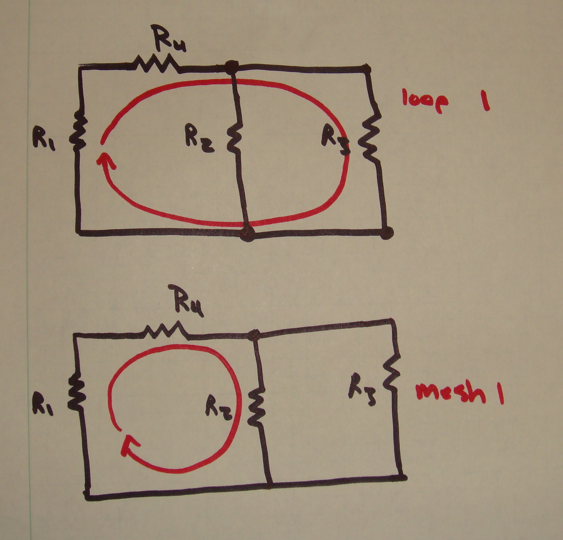
Figure 1. A current loop versus a proper mesh.

It is important to note that a current source along the outside of the loop will ultimately avoid the need of a mesh equation. Also, a voltage source will not effect the identification of the circuit meshes.

Equipment and Supplies

The equipment and supplies listed below are suggested, but other suitable supplies can be used.

·      TI-84 graphing calculator.

·      Engineering or graph paper.

·      Pen or pencil.

 

Mesh Equations Method and a Simple Resistive Circuit

A simple resistive circuit is one where no embedded current sources are present and therefore no super-mesh equation will be developed.

            Identifying meshes. In order to start writing mesh equations, one must identify all meshes in the circuit.

            1. Draw loops around each mesh present.

            2. Establish a counterclockwise or clockwise convention for your mesh currents.

3. Label each loop with a subscript number I as depicted in Figure 2 below for organizational purposes.

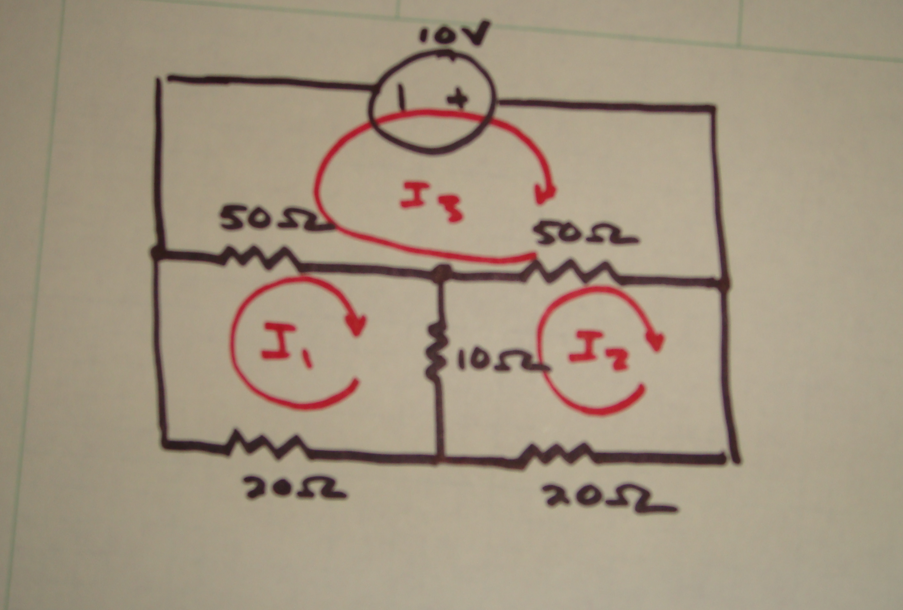
Figure 2. Identification and Labeling of mesh currents.

            Developing mesh equations. Each mesh has a KVL equation associated with it. The total number of mesh equations is equivalent to the number of meshes identified minus the number of current sources. This process assumes no super-mesh is present [1].

            1. Identify the resistors in a mesh.

2. Write the voltage drop across the resistor as I_nR, where I_n is the mesh current and R is the value of the resistance given in the problem.

3. Write the voltage drop across a voltage source as the voltage given in the schematic.

4. Calculate the KVL equations for the mesh. The mesh equations for the circuit depicted in Figure 2 are shown in Table 1 below.

 

 

Table 1. Developed mesh equations based on Ohm’s Law and KVL.

5. Simplify the calculated mesh equations as shown in Table 2.

·      Move all constants to the right side of the equations.

·      Distribute and simplify in such a way that all mesh currents are independent in the equation.

 

 

Table 2. Simplified mesh equations.

            Solving mesh equations. The mesh equations can now be solved algebraically by hand, or with the use of a scientific calculator. The following will only show how such a process is done on a TI-84 graphing calculator.

 

It should be noted that solving simultaneous equations involves the manipulation of matrixes. As a result, the number of meshes determines the dimensions of the matrixes. For example, if there are three mesh equations, there will be three rows in the matrix. Also, if there are three mesh currents there will be four columns in the matrix. Note the addition of the extra column.

            1. Press the 2^nd button followed by the button labeled with x^-1 button.

            2. Scroll to EDIT using the arrow keys and select the first option, matrix [A].

            3. Enter the matrix dimensions based on the number of mesh currents and mesh equations.

4. Enter the coefficients to the mesh currents into the rows of the matrix. Start with the first mesh equation.

·      Every equation will occupy one row in the matrix.

·      Every index in the matrix must be filled. If the mesh current is not present in a mesh equation, enter a 0 for this coefficient.

·      Enter the constants on the right side of the mesh equations in the last index of the row.

5. Press the 2^nd button followed by the mode button to return to the home screen.

6. Press the 2^nd button followed by the x^-1 button and scroll to MATH section using the arrow keys.

7. Press the ALPHA button followed by the APPS button.

8. Press the 2^nd button followed by the x^-1 button and select the first option, matrix [A].

9. Press ENTER and the magnitude of the mesh currents are shown in the last column of the resulting matrix.

Source

[1] Lakdawala, Vishnu. Ece 201. Class Lecture, Topic: "Mesh Equations Method." KAUF 224, Old Dominion University, Norfolk, Virginia, Fall 2008.